Measure a MAS rotor
Dataset Information
Filename: MAS-rotor_{650,650,515}_uint16.bin
volume = {650, 650, 515}, x-fastest, pixel size = 5.67 µm, file size = 415 MB
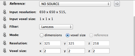
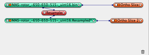
Downsample the dataset
- Launch Avizo 7, file->Open data as, choose the rotor binary dataset, click open, in the popup window, choose RAW data, click ok, input correct dataset inforamtion (650x650x515, x-fastest, little endian), click ok to load data into Avizo. A data object icon will appear in the object pool. Attach Display->orthoslice to visualize (left-click to choose the data object, then right click to choose the orthoslice module).
Review the full dataset
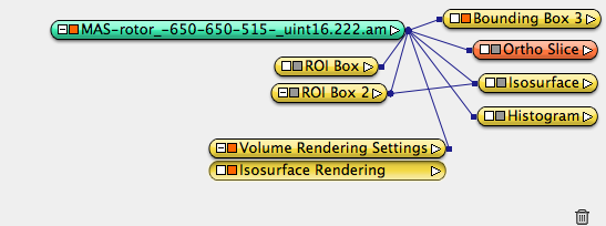
Delete the original binary data object, reload the downsampled .am data object, attach orthoslice to visualize.
Inspect data value: orthoslice data window, histogram, isosurface.
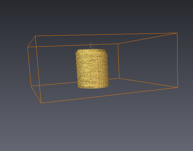
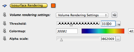
Right click on data icon, choose Display->Isosurface Rendering, set Alpha scale to 0.1, tweak the threshold value to see the result.
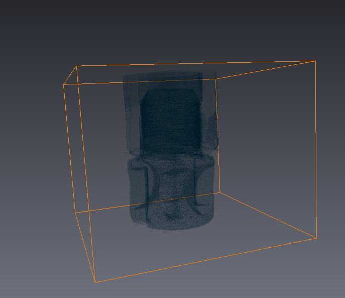
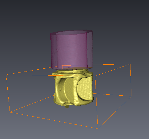
Notice the dataset has two parts with different data value characteristics. Duplicate the dataset twice (both from the original data object), crop each one accordingly so that the two parts are separated data objects: part I and part II.
Reconstruct Part I
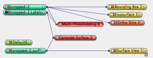
On cropped data object part I, visualize the dataset by bounding box, ortoslice, isosurface.
Optional: On data icon, right click and choose Image Filters->Smoothing:Median, choose 3D operation, apply.
Optional: On data icon, right click and choose Measure->Line Probe, choose yz orientation, set sample number to be 200, click show button to show the line profile. Now change the data entry of the line probe to be the median filtered data object, observe the difference of the line profile.
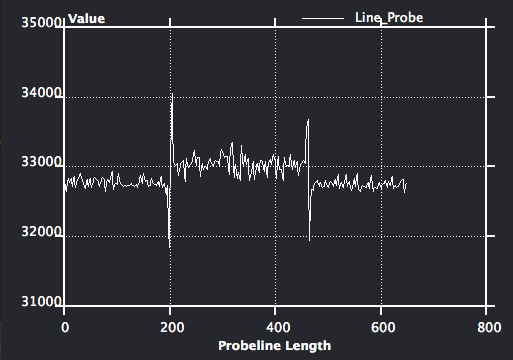
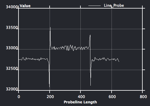
One data icon, right click and choose Image Segmentation->Multi Thresholding, edit to three-materials mode (delete the “bone” lable in Regions input), so only two threshold levels are present. put 33000 and 38000 as threshold value, apply, a .lables data object will be created.
Examine the material labels, Delete materials not of interest. Leave only the background(exterier) and the rotor(fat), rename material name from “fat” to “rotor” by double clicking on the name of material. While choosing the rotor material, right click and choose draw style -> 3D View, to see the 3D structure on the perspective window (upper left corner).
On menu->Segmentation, choose Remove Island, then Fill Hole. Thesegmentation should be relatively clean.
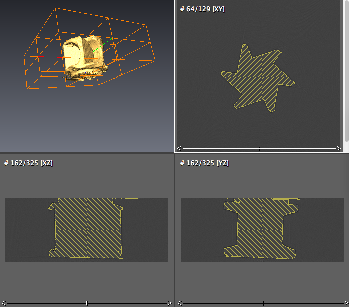
- Click the .label data object, choose Compute->Generate Surface to generate surface, Apply, a .surf data object is created. Use the simplifier icon to simplify the surface if desired. then use Display->Surface View module to visualize.
Reconstrcut Part II
- On cropped data object part II, visualize the dataset by bounding box, ortoslice, isosurface.
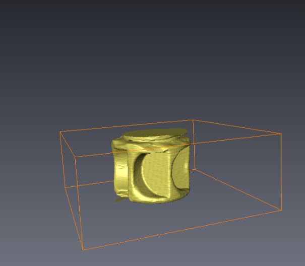
- One data icon, right click and choose Image Segmentation->Multi Thresholding, edit to two-materials mode, so only one threshold levels are present. put 36000 as threshold value, apply, a .lables data object will be created.
- Examine the material labels, Delete materials not of interest. Leave only the background(exterier) and the rotor(fat), rename material name from “fat” to “rotor” by double clicking on the name of material. While choosing the rotor material, right click and choose draw style -> 3D View, to see the 3D structure on the perspective window (upper left corner).
Reconstrcut Part III
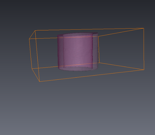
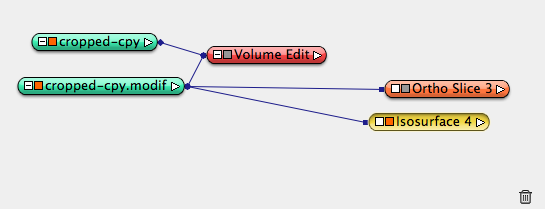
Duplicate cropped data object part II, rename it cropped data part III. Apply Compute->Volume Edit, in Tool sectin, choose tab box, cylinder, line, and z axis, interactive adjust the cyclinder radius until an inner circle of the part II is picked, apply. A new .modif data object is created.
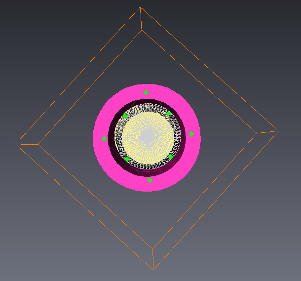
Apply isosurface to .modif data to reveal Part III. Similar steps to generate surface can be applied the same as part I and II.
