Segmentation of basalt datasets
Note
Filename: GL01_6_28k_resampled.222.am
Pre-Processing
- Open data in Avizo, use orthoslice to visualize, also try other display modules, such as isosurface, volume rendering, etc. Have a look of the dataset.
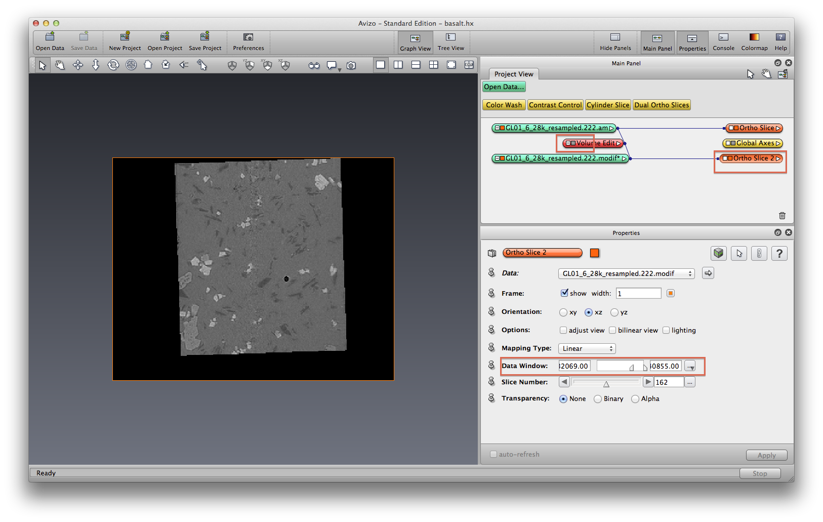
- Use orthoslice data window to find proper threshold data values for different mineral phases. How many mineral phases you can find?
- Does De-Noise filtering help? Apply smoothing filter to remove noise before proceed to segmentation. In this example, I used ImageFilters->Smoothing:Edit-Preserving with default parameters, apply. A .filtered data object will be created. I didn’t find too much improvement from the smoothing filter.
Data Transform
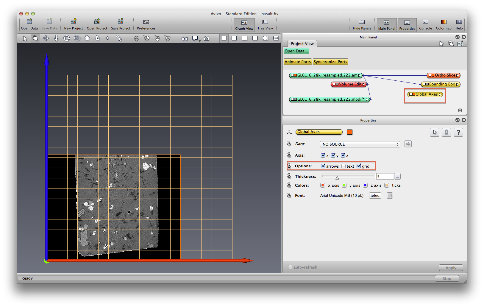
Switch view mode to Orthographic, select orthoslice orientation as XZ, On Menu bar, choose View->Axis, turn on arrows and grid optoins. You can see that the data is tiny bit tilted.
If you want to transform the data directly, click on the basalt data object icon, in Properties panel, click on Transform Editor icon, switch mouse to interactive (arrow) mode, grab the right green tab to rotate the sample until mostly straight, use the grid line as guidance. You can do this in YZ direction as well.
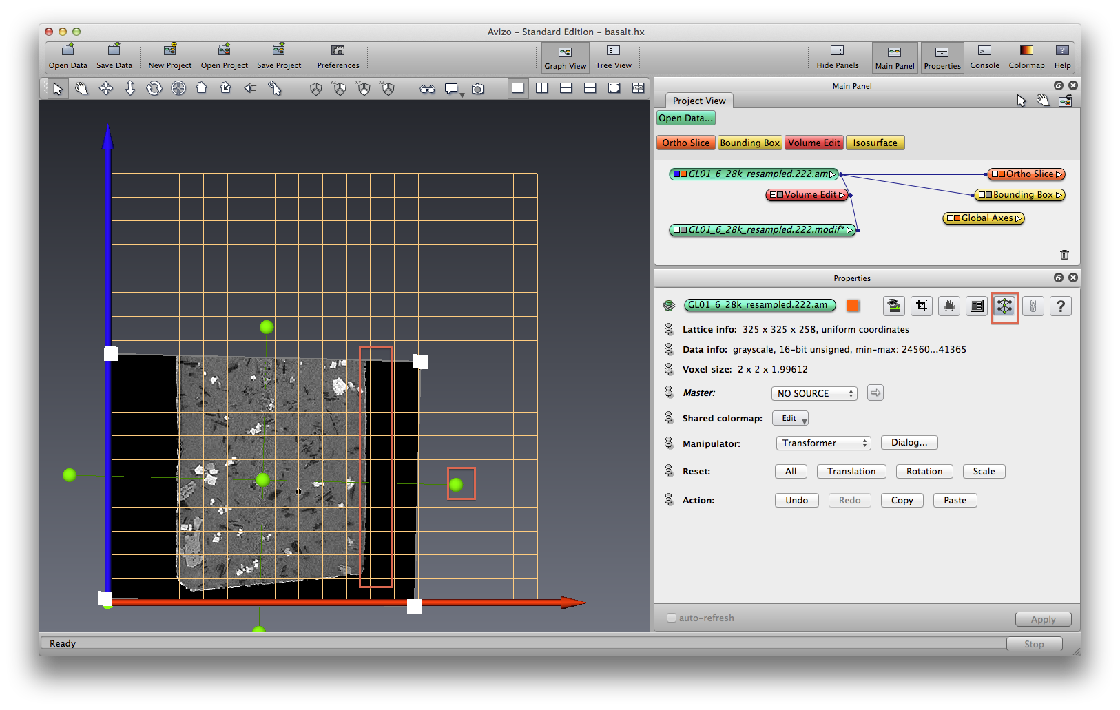
In this tutorial we will not transform the data directly, so click the “All” button in “Reset” section. click on Transform Editor icon again to turn off the editor mode.
Edit volume
Right click on data object, choose Compute->Volume Edit. In Properties panel, find Tool section, set the options as: TabBox, Cylinder, Lines, Z axis. Switch view mode to Orthographic, select orthoslice orientation as XY, switch mouse to interactive (arrow) mode, click and drag the transform box to resize the cylinder until it only covers the basalt sample. I make it slightly smaller than the basalt sample so I get rid of the edge problems. Switch orthoslice to XZ direction, change volume-edit to Transformer tool, tilt the volume edit cylinder a little bit. Switch back to TabBox tool, make the size more fit inside the sample.
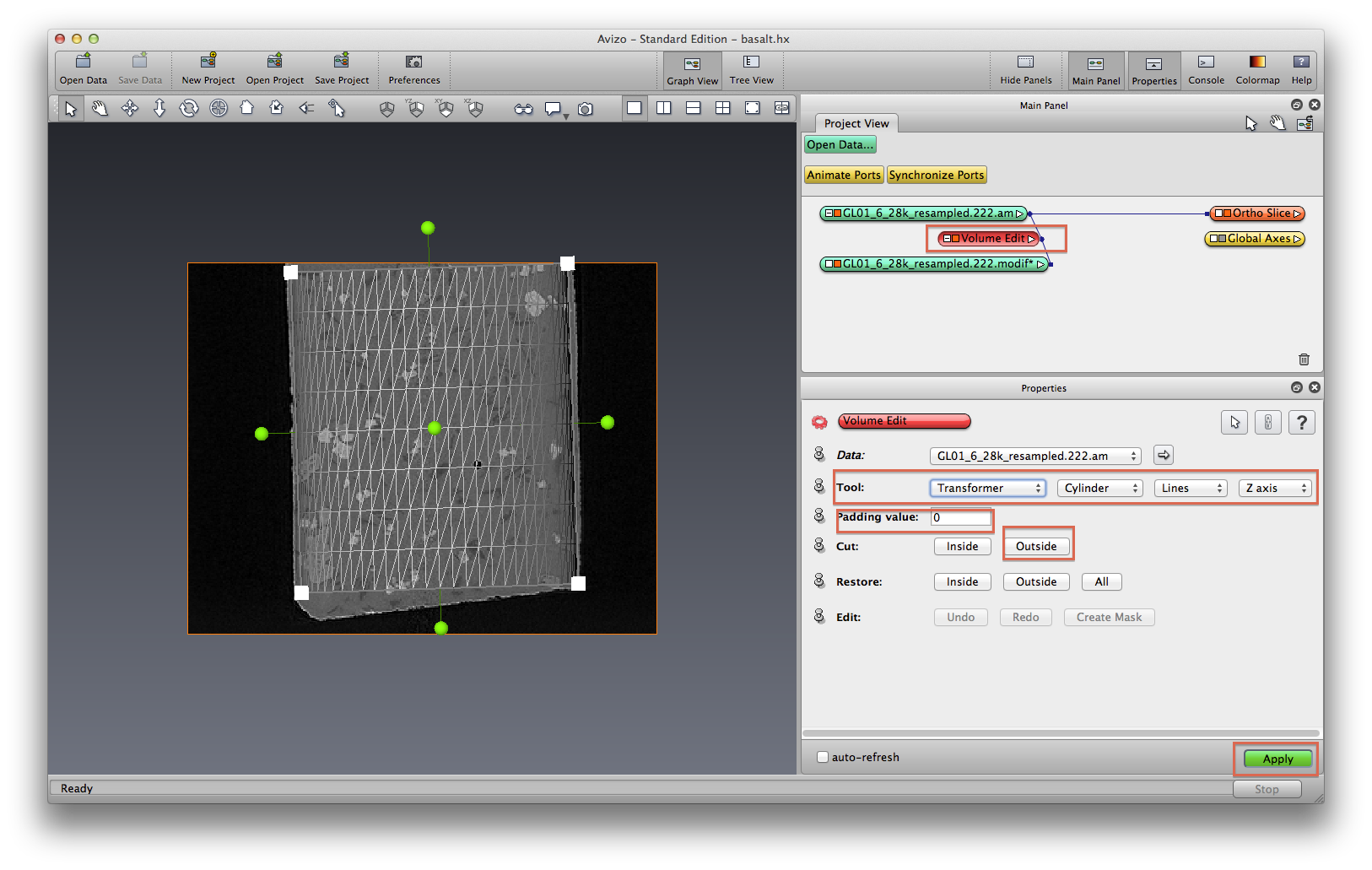
After you are happy about the cylinder coverage, click Outside in Cut section, set padding value to 0, click Apply. Use orthoslice to visualize the modified data. You will see by default the orthoslice looks much whiter, this is because we padded the outside of volume edit cylinder to value 0, now Avizo knows the minimun data value is 0, so it plotted using the current min-max data value. In retrospect, maybe we should use a padding value such as 30000. Hide Volume Edit module by clicking on the small color block.
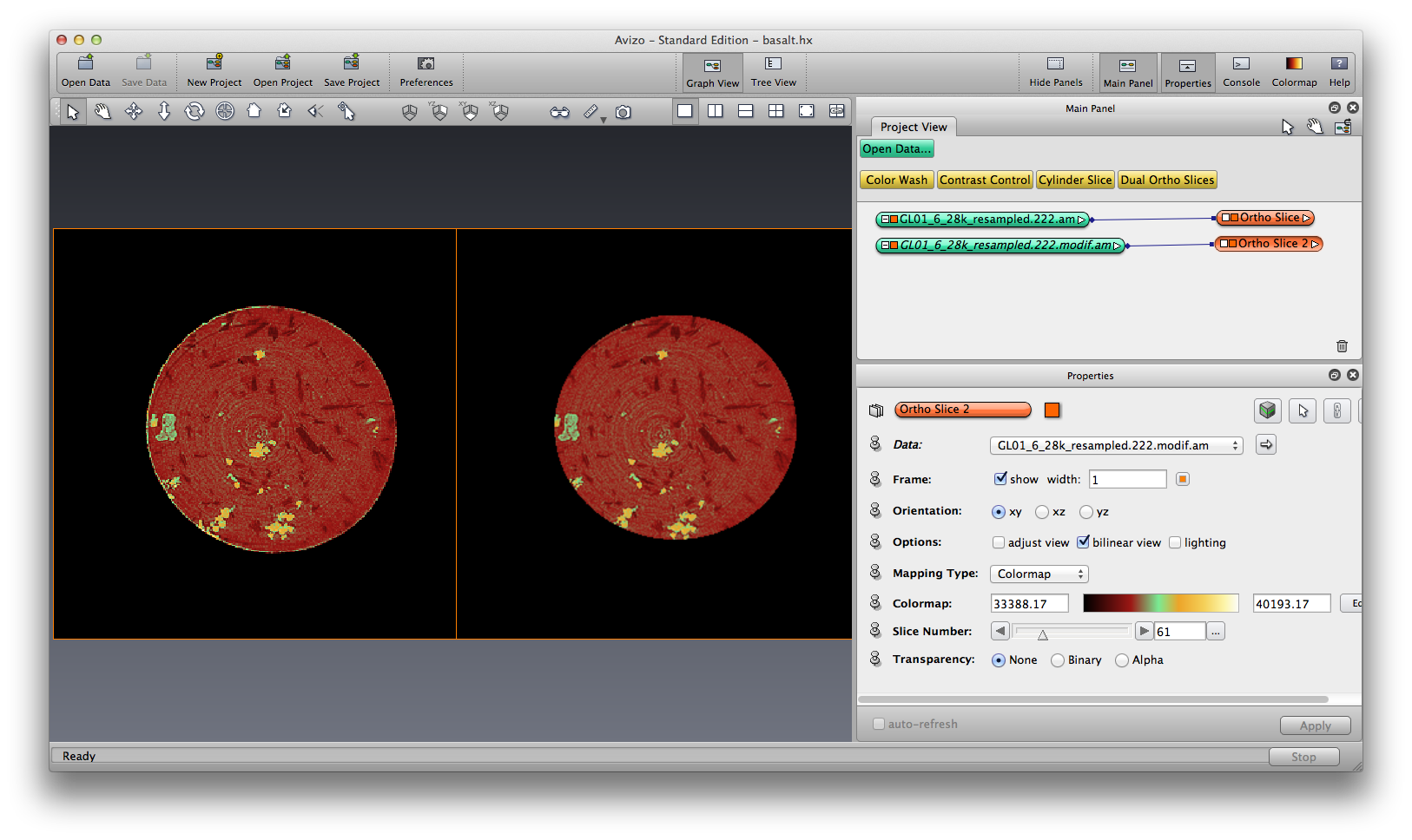
Now we plot the origial and volume-edited data in orthoslice side by side, this is done by tranform the volume-edited data to the right side (translate) using the Transform Editor. Also use a colormap to show the orthoslice, make it look like a mineral phase element map.
Segmentation
In this tutorial we segment one phase at a time, intead of trying to segment multiple phases at once.
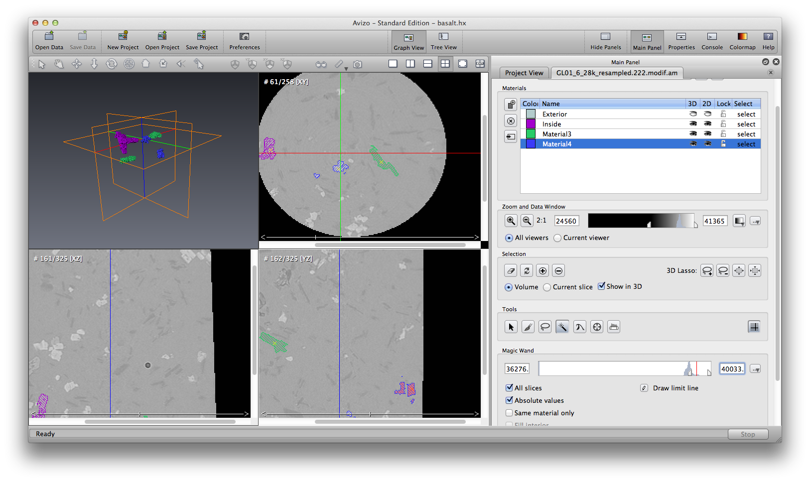
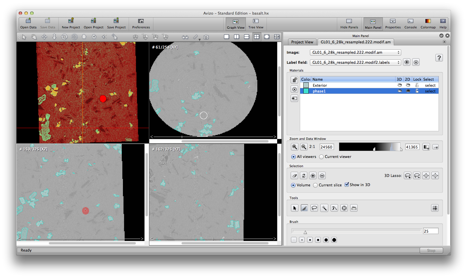
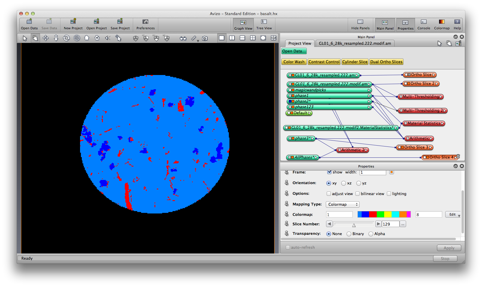
Let’s use segmentation editor to look at the phases first. Right click the data object, choose Image Segmentation->Create New Label Field, this will create a .labels file for you. Click on the .labels file, invoke segmentation editor, use magic wand to choose a couple of phase minerals and assign them to different materials, see the below screenshot as an example. Here I want to make clear a concept, that segmenation means “label” your data, not “binalize” your data. Binalization is a speical case of labeling.
Right click the data object, choose Image Segmentation->Multi-Thresholding, set Regions to be “exterior phase1”, set threshold value: 36000, apply. Another .label data object is created. click the new .label data object, then click the Image Segmentation icon in the Properties panel to open the segmentation editor. Delete the “bubble” meterial. Assign different colors to materials if necessary. To get a good threshold value, I usually use orthoslice data window, or magic wand in segmenation editor, to help me identify good threshold value candidates, then fine tune them by re-running multi-thresholding module and check results.
In segmentation editor, use zoom icon in “Zoom and Data Window” section to adjust window size. Use the “cross hair” tool to connect the three cross sections. Use “brush” or “magic wand” tool to manually fix individual selections in “phase1” material where you see fit. Manual segmentatin is very tedious but sometimes absolutely necessary.
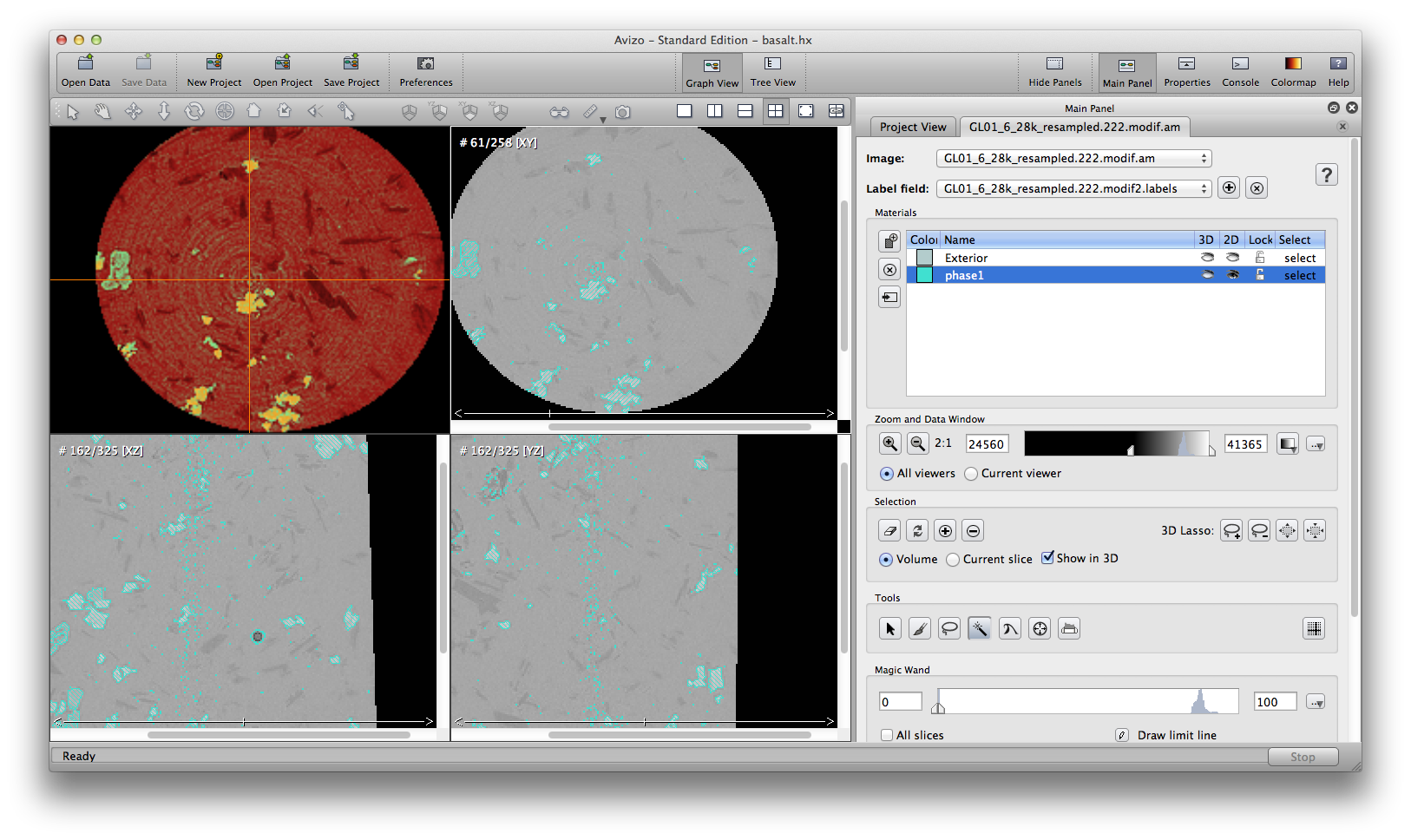
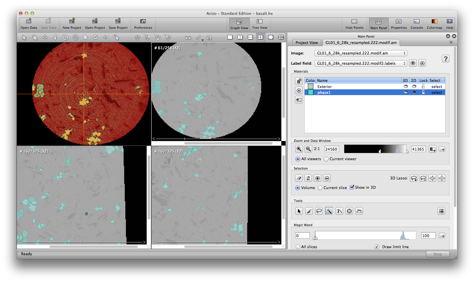
Some automatic segmenation you can do from the menu: segmentation->fill holes, remove islands, and smooth labels. You can choose to apply these commands to either single slice, all slices, or 3D volume. Be careful tho, these commands are not reversible, there is no “undo” button. So it’s a good practice to save the .labels file, or save project, before you try automatic segmentation tools. The below screenshots show the original phase1 material, result after remove island, and result after fill holes.

Another important semi-automatic method is interpolate selection through multiple slices. In the following example, we’ll remove some noise around the air bubble in phase1 material. Scroll up and down inside the xz orientation window, I see slice 159 to 164 contains the noise I want to remove. At slice 159, use the brush tool to mark a selection on the desired area, go to slice 164, do the same, then choose from menu: selection -> Interpolate. Scroll up/down to check the slices, you will see slices 160, 161, 162, 163, all automatically have selections marked because of the interpolation from slice 159 to 164. You can delete the selection from the current phase1 material now.
Right click the label data object, rename to phase1. Save the label field data by file -> save data as, save to Avizo data format, or Raw data format. The segmentation result is the .label file.
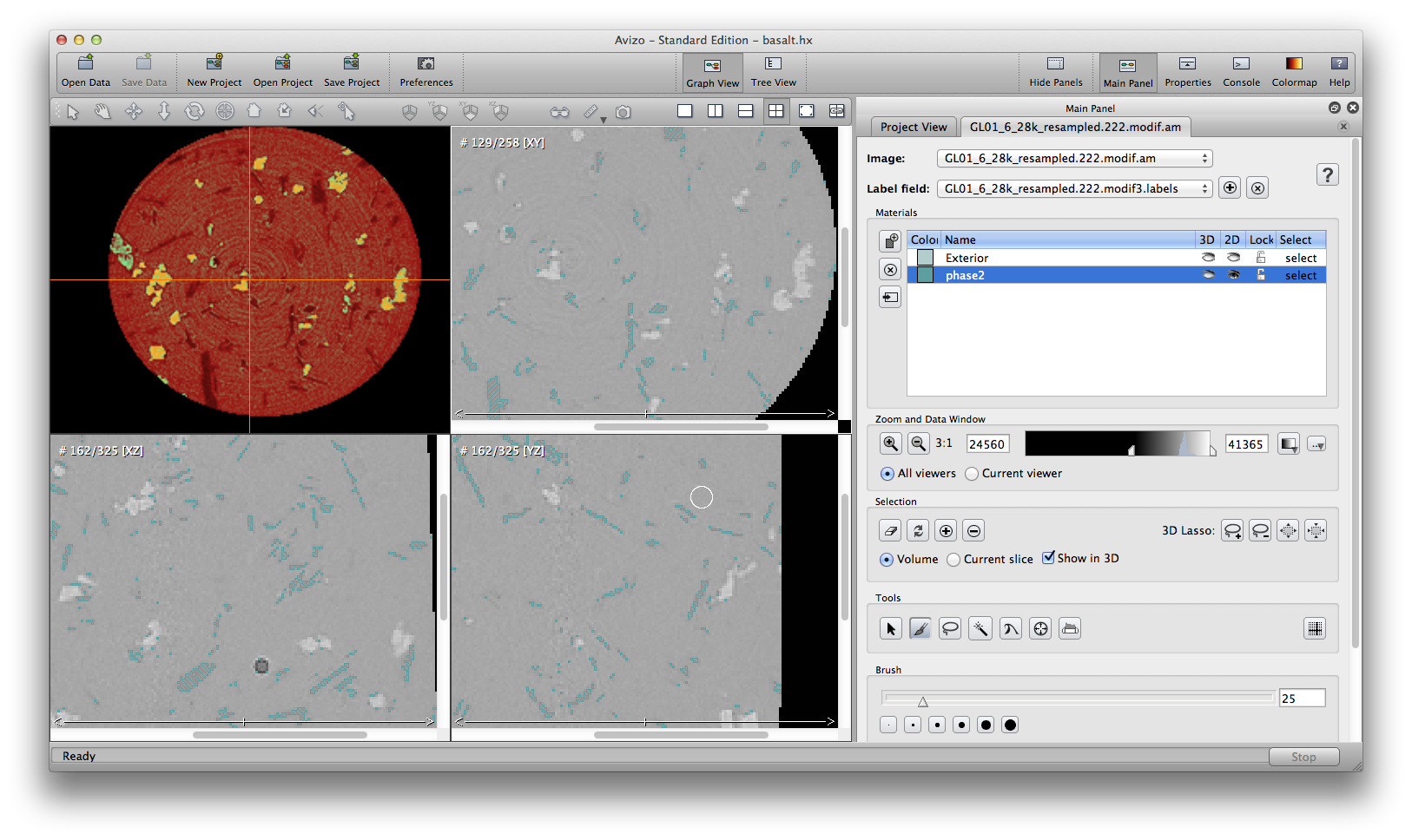
Now let’s do the second mineral phase. Click the data object, choose Image Segmentation->Multi-Thresholding, set Regions to be “exterior phase2 other”, set corresponding threshold values: 34000, 35000, apply. A .label data object is created. click the .label data object, then click the Image Segmentation icon in the Properties panel to open the segmentation editor. Delete the “other” and “bubble” meterials, and keep meterial”phase2”. phase2 material is thin, with lots of small features. This is partly because I down-sampled the original basalt dataset to a much lower resolution. So be careful, if you use “remove island” on phase2, you will end up removing most of small features in phase2. I decided no to do any automatic operation here. Rename/save phase2 label if you want.
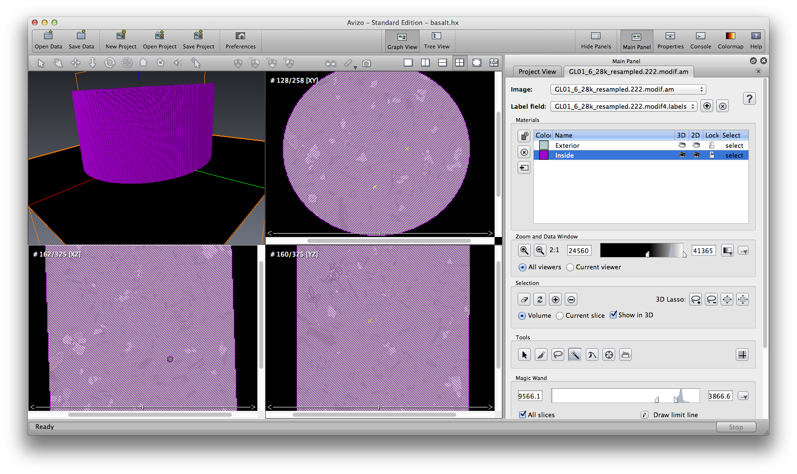
Next step, right click the data object, choose Image Segmentation->Create New Label Field, use magic wand to choose the whole basalt area, and remove the air bubble. This material includes all mineral phases, I name it phase123.
Now we have phase1, phase2, and phase 123, we obtain phase3 by doing a simple Arithmetic operation, phase3 = phase123 - phase1 - phase2.
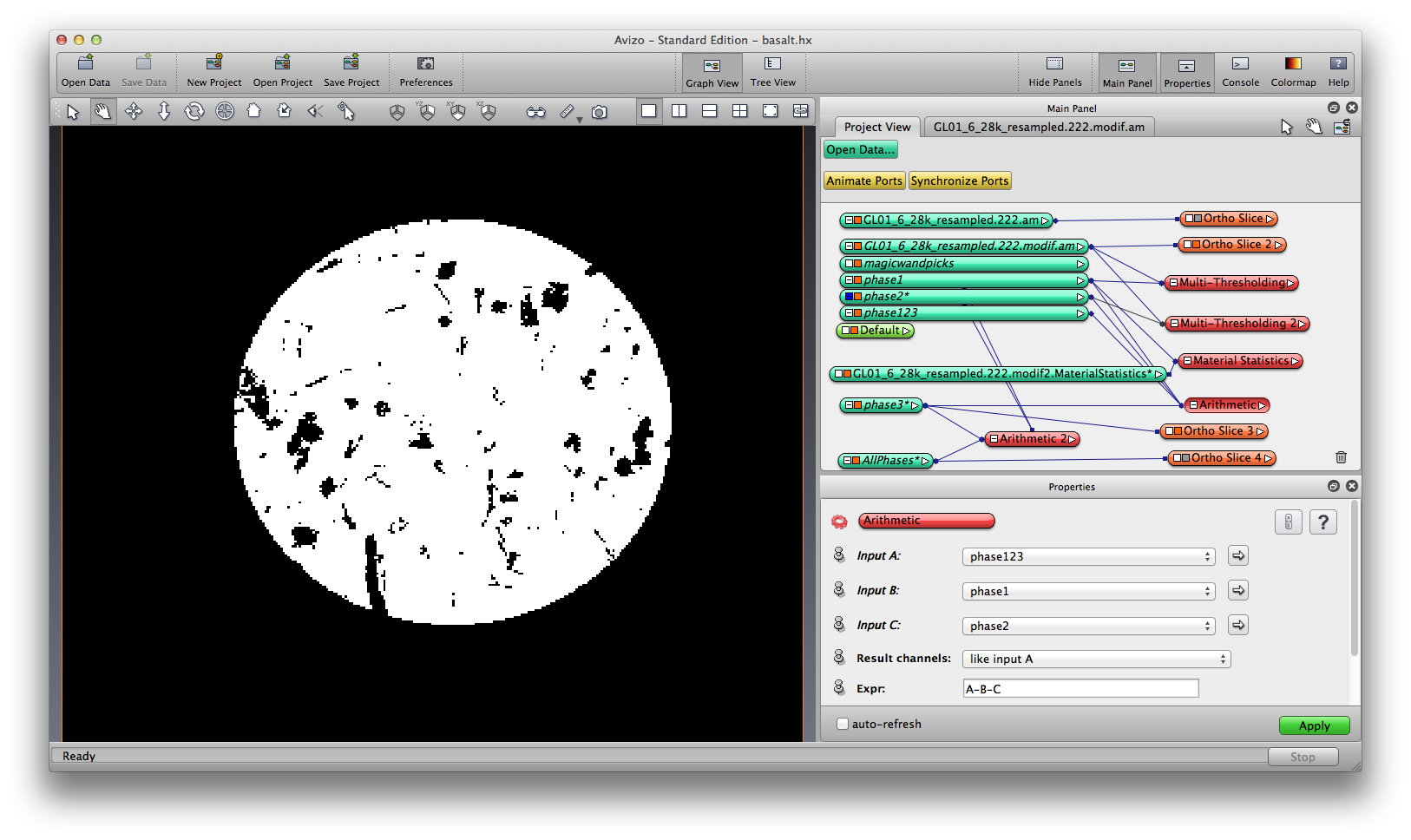
Because we choose to segment one mineral phase at a time, now we have three separate label field, each of them mark one mineral phase, by data values 1. Now we’ll merge the three label fields into a single label field, so the mineral phases are marked by data value 1, 2, and 3. Again we use the the compute -> Arithmetic module with three inputs and expression as ”A | (B*2) | (C*3)”. Now you can visualize the three mineral together. Save the merged label data.
Now you can visualize the labels, by generate surface and surface view, volume rendering, isosurface rendering, etc.
Measure the three phase label field by Measure -> MaterialStatistic.
Note: We segment on the assumption that there are three mineral phases. There actually could be more phases. For example, data value range 36000 to 37000 and data value above 37000 could be two phases, whereas here we include them both as phase1.