Measure a bullet’s cartridage and propellant grain size and distribution
Note
Filename: volume_bullet_p134_uint16.bin
volume = {243, 243, 227}, z-fastest, pixel size = 55 µm, file size = 27 MB
Measure the cartridage volume using manual measuring tools
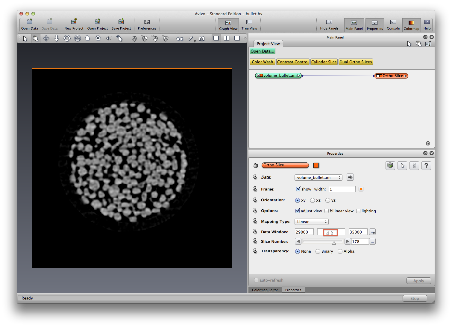
Launch Avizo 7, file->Open data as, choose the bullet binary dataset, click open, in the popup window, choose RAW data, click ok, input correct dataset inforamtion (243x243x227, z-fastest, little endian), click ok to load data into Avizo. A data object icon will appear in the object pool. Attach Display->orthoslice to visualize (left-click to choose the data object, then right click to choose the orthoslice module).
Right click on data object icon and save data as Avizo format (.am), so next time you don’t need to input the file information again.
Attach Measure->Histogram module to the bullet data object, click Apply, a histogram window will show up, which tells you the data value distribution of the bullet dataset.
Choose the ortho projection mode, use the measure tool (top layer tool icons, look for the ruler shaped icon) to measure the diameter and height of the cartridge in pixels, multiply by pixel size (55 µm)

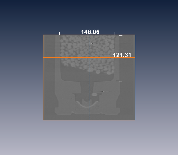
Compute the volume as: bullet-volume = pi * radius * radius * height
File->Save Project As, to save the project. Next time you can just open the project and the visualization network will be restored.
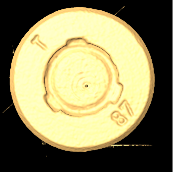
Check the bullet marking on the bottom by isosurface
Attach Display->isosurface module to the bullet data object, set threshold (slider) to 28000, apply. Rotate to the bottom of the bullet, the marking would be readable
Tune the threshold value to other values, such as 31000, look at other geometry features
Do Display->ROI Box to selet a region of interest, and use it as data source of the isosurface module.
Visualize the bullet structure using Volume Rendering
Attach Display->Volume Rendering module to the bullet data object. Hide the Orthoslice module in project view network, so we only look at the volume rendering itself. Make the visualization smaller by zooming out a bit, volume rendering is computationaly expensive, less visualization pixels may speed up the rendering for you.
In Properties panel of Volume Rendering module, look for Colormap item, click the Edit button, choose volrenWhite.am as the default colormap. There are two text input boxes where you can set the data value limit (min,max) for volume rendering computation, set min value to 27000, press enter in keyboard, see the rendering changes.
In Properties panel, look for Colormap lookup item, change from rgba to alpha.
In Properties panel, look for Alpha scale item, set value to 0.25.
Play with different properties settings, try to understand how they reflect to the rendering changes.
Now let’s customize the colormap to what we really want for this dataset. First change Colormap lookup to rgba, then click the Edit button in Colormap item, choose Options->Edit colormap..., the Colormap Editor window will open, drag it around and resize Avizo window layout so we can easily edit the colormap and see the rendering updates. For later steps, refer to the screenshot below for spots to click on.
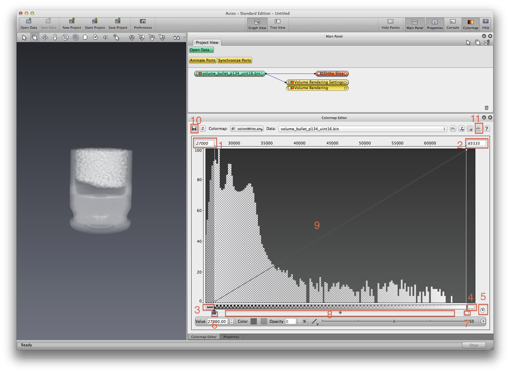
Click on spot 1 and 2, to edit min-max value, same effect with step #2.
Click on spot 3 and 4, to set color for data value out of min-max limit.
Click on spot 5, to expand the key point edit panel. You can edit data value, color (RGB) and opacity (alpha, A) at a selected key point. There are two types of key points: color and opacity. For any type of key point, left click to select, drag to move, and right click to delete.
Click on spot 6 and 7, to set color (RGB) for min-max color key points.
Click anywhere underneath color bar, in area 8, to add a new color key point, edit color details in key point edit panel.
Click anywhere in the graph area 9, to add a new opacity key point, edit opacity details in key point edit panel.
Explore the colormap editor more, see the visualization updates. If you want to save this colormap you just edited, click spot 10 to invoke the save file dialog, save to a new name, inside your project file folder.
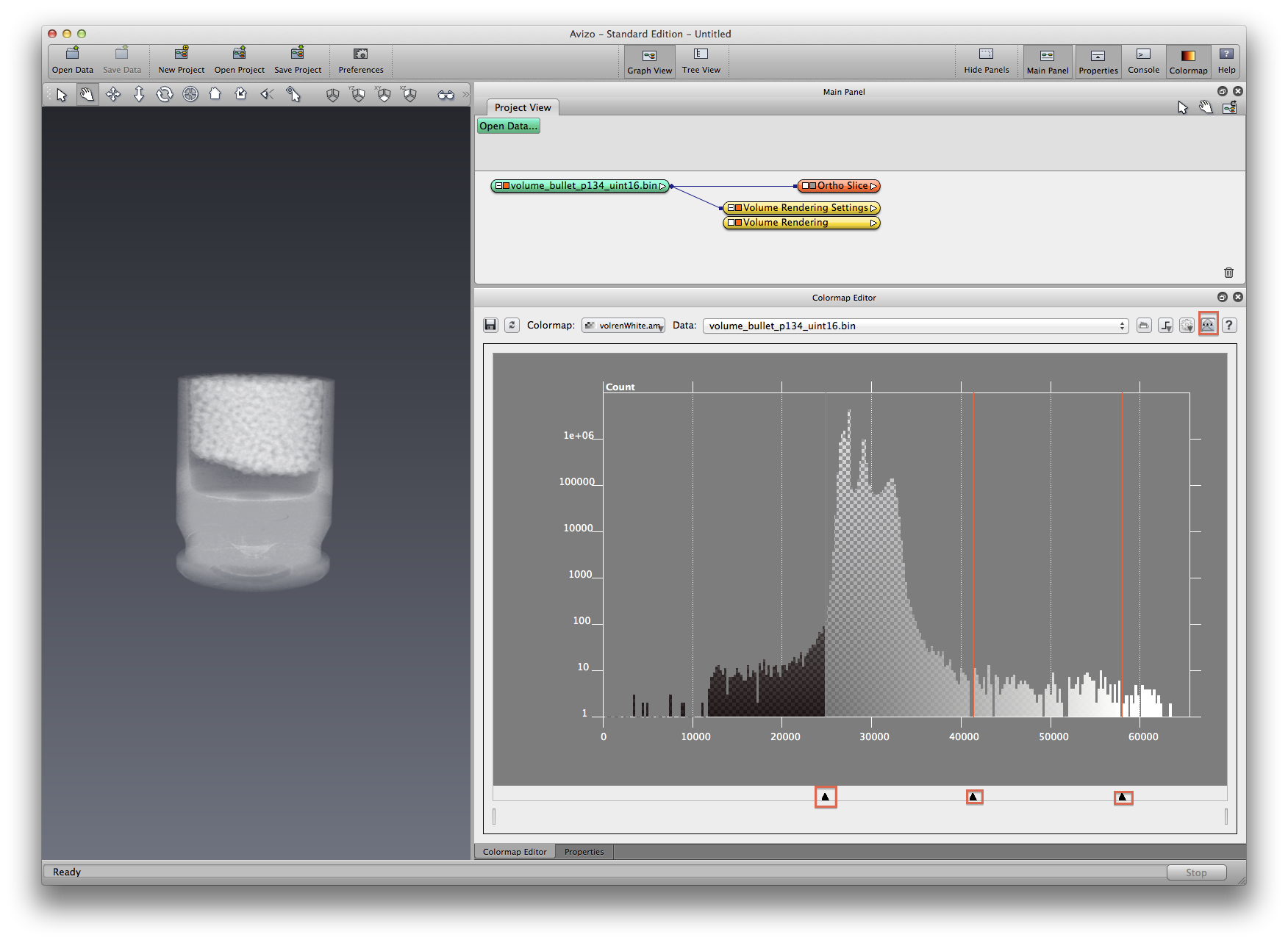
Click spot 11 to switch to data range view, drag the three black triangles (see screen shot below) to change the colormap applying range.
Save the project, choose autosave to save your customized colormap, and any new data you created for that matter.
Measure the propellant volume and surface area by isosurface
Open data, use isosurface with value 31000 to reveal the propellant structure.
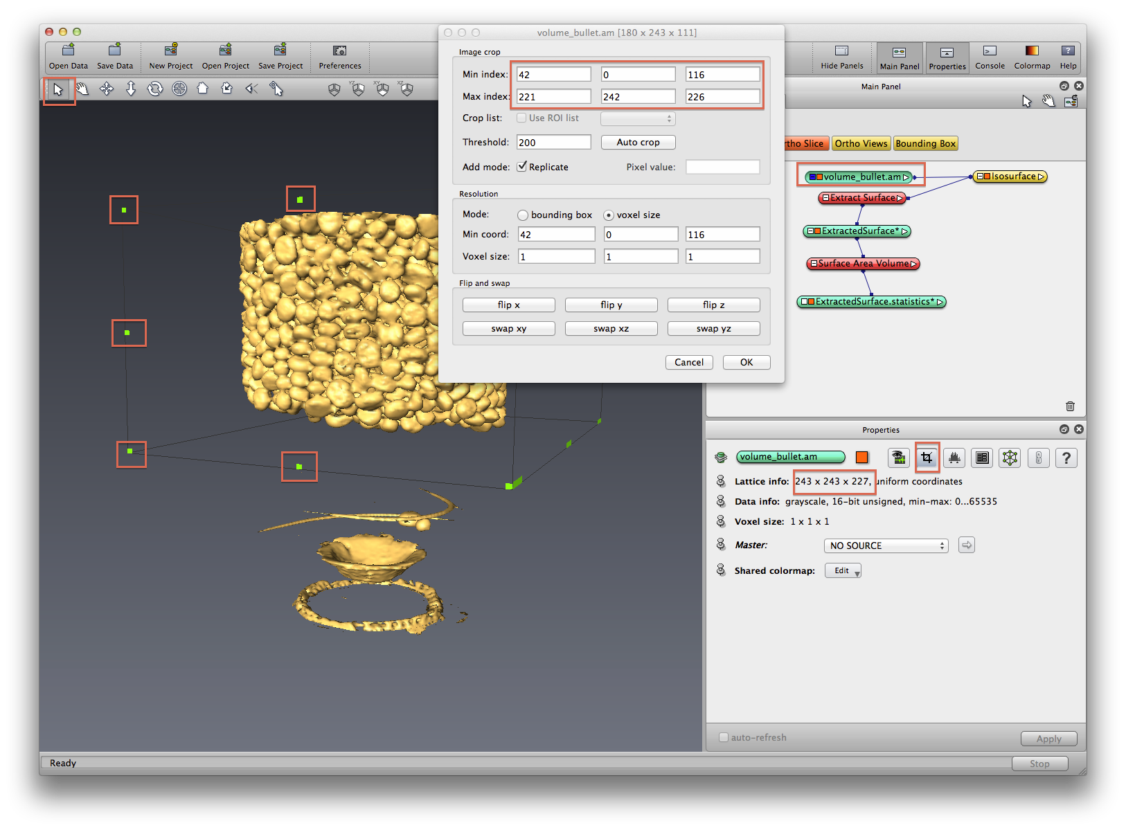
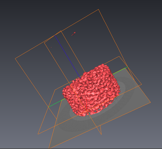
Right click on data object, choose Object->Duplicate Object, exercise crop data on the duplicated copy. See below screenshot. Right click Object->Rename to rename the cropped dataset. If you don’t see your isosurface updated after crop, delete the old isosurface module and redo it.
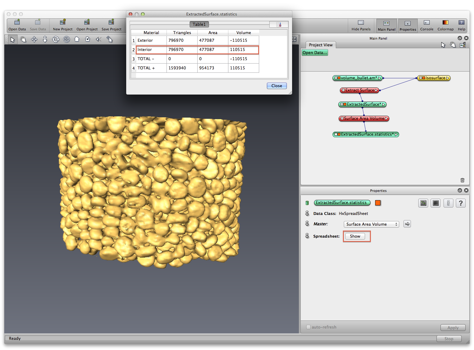
Right click on isosurface module, choose Extract Surface, Apply. An ExtractedSurface data object is created, right click on it, choose Measure->Surface Area Volume, in Properties panel, click show button to show the statistics as a spreadsheet.
Right click on ExtractedSurface data object, choose Save Data As, save it as a .surf data, which you can open separately later. Save your project.
Measure the propellant volume by segmentation
Use Isosurface to extract and measure a feature is easy and convenient, but it only works on very clean dataset, with very limited capability. What we want for our bullet project, is to separate each propellant grain, count their numbers and measure their volume individually. To do this kind of work, we will use segmentation tools and label our data first.
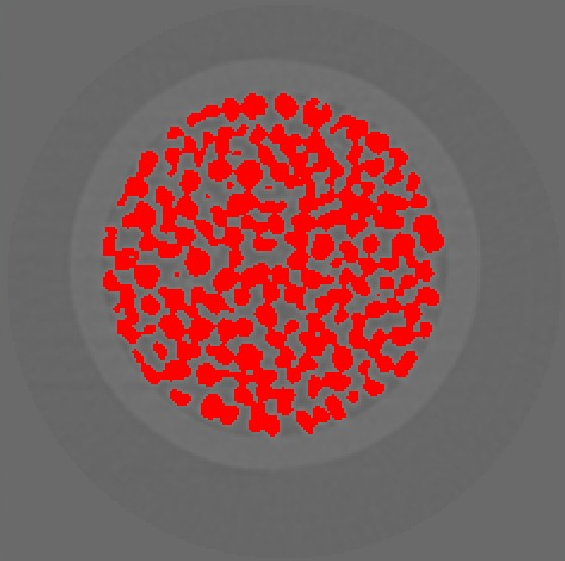
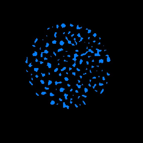
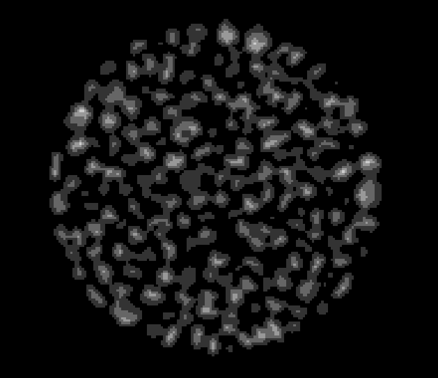
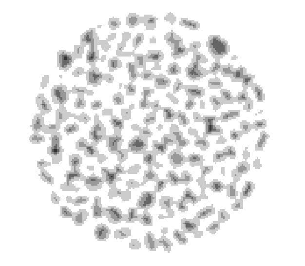
Open data, attach orthoslice to visualize slices, tune data window in orthoslice Properties panel, drag left and right side markers (min-max value) until the slice looks all black but the grains, go through all slices and check.
Explain terms: threshold, binarize, label. Find good threshold values are very important, because we will use these threshold values to segment our bullet dataset.
On data icon, right click->Image Segmentation->Multi-Thresholding, in Properties panel, set Regions to be: Exterior grain other, then hit enter in keyboard. Choose threshold set: 31000, 35000, click Histo button to show histogram with the threshold value, click Apply. A label field data object datasetname.labels is created, take some time to understand what’s the difference between the label field data and the original data. The Properties panel has some helpful information.
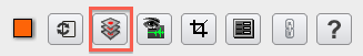
Choose the .labels data object, invoke segmentation editor by clicking the segmentation icon in the property panel. The view window will be split into 4-view mode.
Examine the material labels, Delete materials not of interest. Leave only the background(exterior) and the propellent(grain). While choosing the grain material, right click and choose draw style -> 3D View, to see the 3D structure on the perspective window (upper left corner).
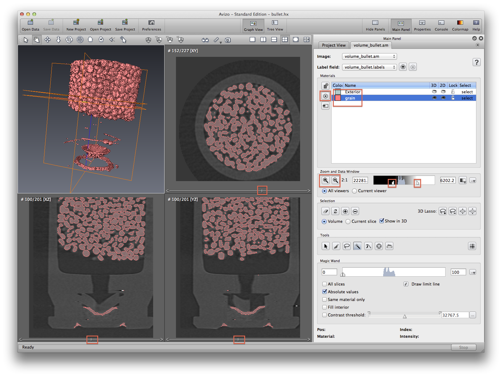
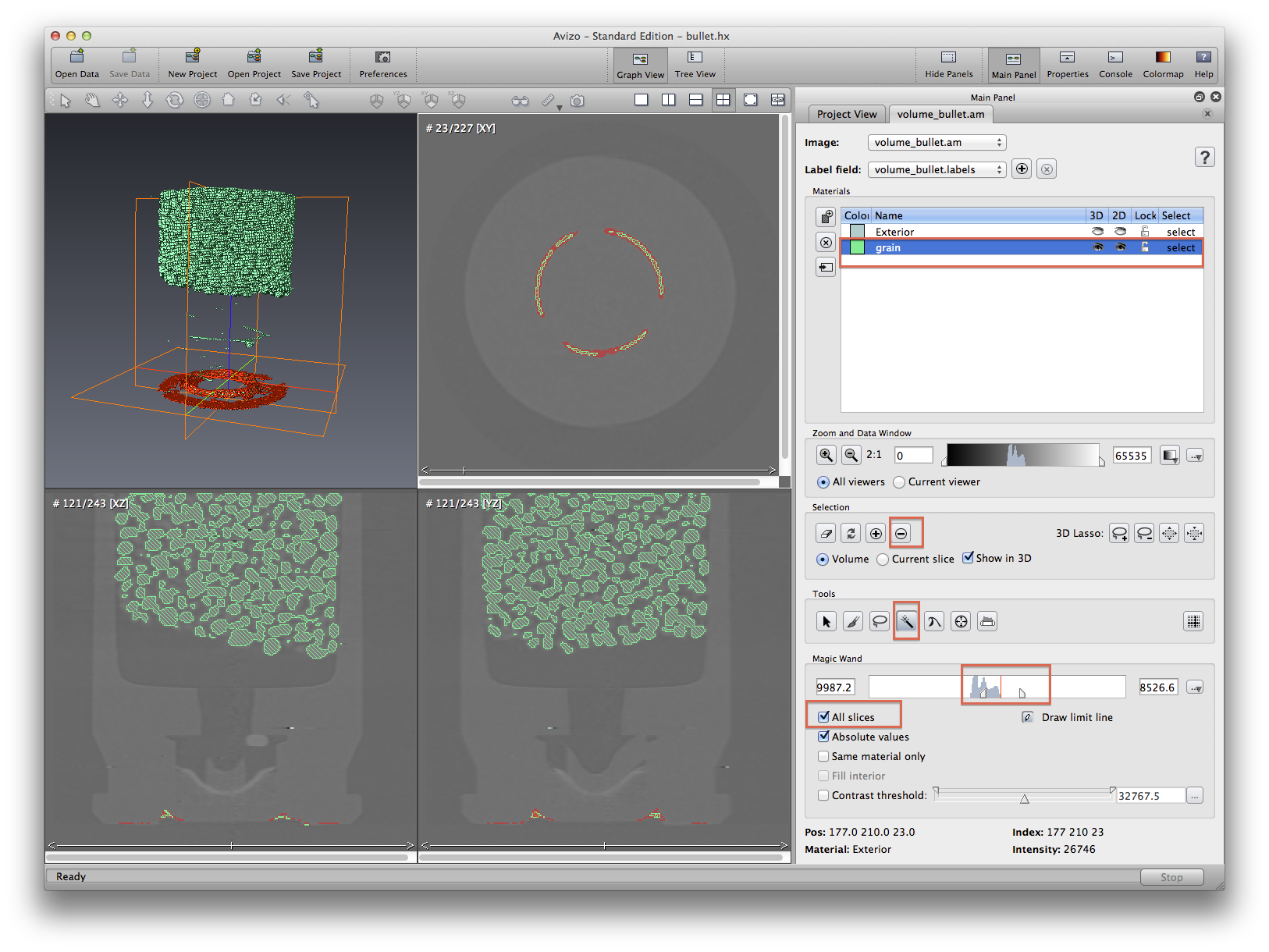
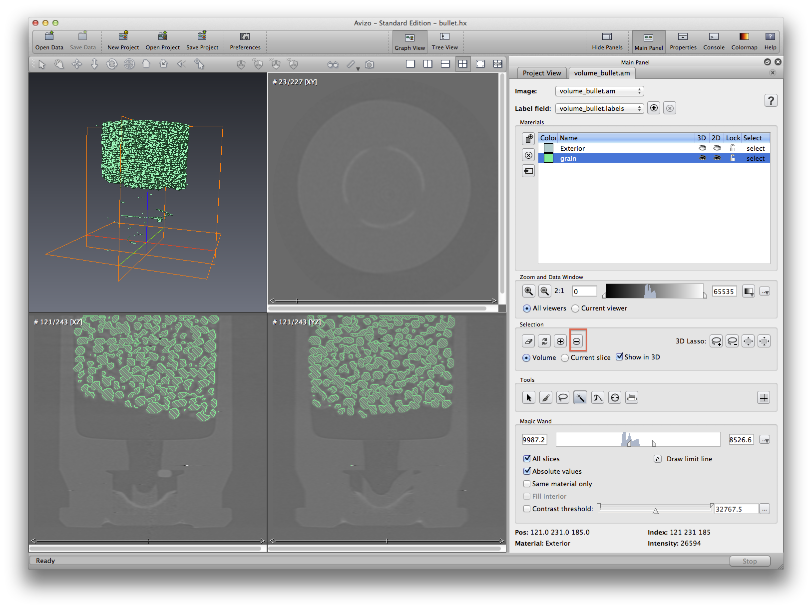
Now we will practice using magic wand tool to remove some unwanted areas from a selected material. See screenshots to see the process before and after. Note that when using isosurface to do measurement, if there are some part of the isosurface you don’t want, you will have to crop the data first. This is not always plausible, because a simple crop may not do the job. But in segmentation editor, you can manually select some part and delete them from an existing material.
All of the grains are still connected, because they are touching each other. We will have to do more image processing to the .labels data object in order to separate the grains. But for now let’s measure the whole grain volume just like we did with isosurface. Go back to the project view tab. Click the .labels data object, choose Measure->material statistics. Apply, a statistics data will be created, select it and click the show button at spreadsheet section. Volume of the propellant will be measured and reported in a spreadsheet format.
Click the .labels data object, choose Compute->Generate Surface to generate surface, Apply, a .surf data object is created. Use the simplifier icon to simplify the surface if desired. then use Display->Surface View module to visualize.
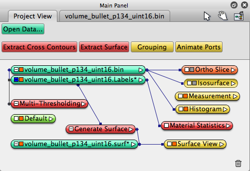
This is the Avizo network:
File->Save Project As, give your project a name, such as bullet, it will be saved as bullet.hx file,Choose “auto save”, save all intermediate data generated by Avizo, especially the .labels data, make sure it is saved.
Segmentation tools are very useful, we will come back to it when we visualize other datasets as well.
Separate the propellant grains by Erosion and Dilation
Open project bullet.hx, Avizo will automatically reproduce the previous work you did last time. Attach Orthoslice to the .labels data object, select the same slice number as the first orthoslice module, use the show/hide trick to check difference between two isoslices. Enable transparency as “Binary” to visualize both the original image and the labeled image. Don’t stress on the color, you may use differenct colormap from what I use here as red.
Right click the .labels data object, choose Image Morphology->Erosion, set Filter to 3D, neighbourhood to 26, size to 1, Apply. A new filtered data object will be created, use orthoslice to visualize. The combination of Filter type, neighbourhood and size parameters creates an image morphology kernel. The goal here is to see the separated grains. If the speration is not good enough, try different kernel setting. This is the easiest way to do geometry feature separation.
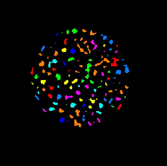
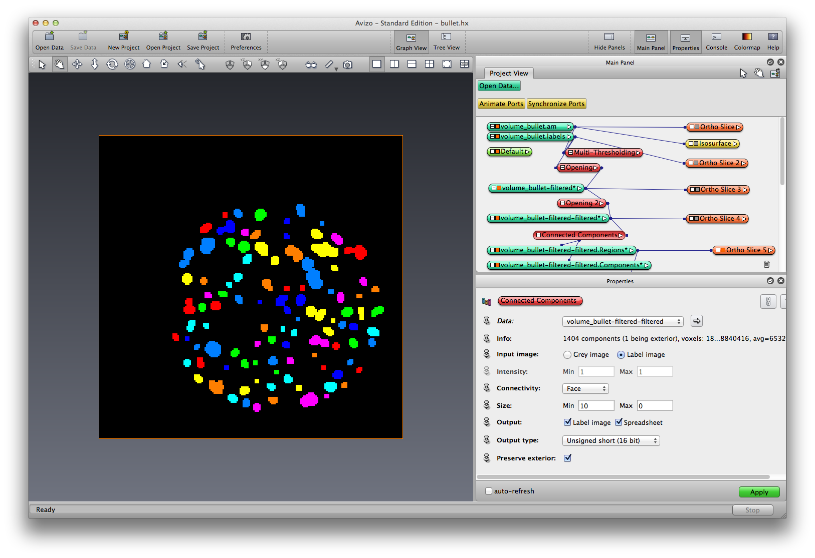
Right click on the eroded data object, choose Image Segmentation->Connected Components, choose input as Label image, output to be both Label Image and Spreadsheet, output label image to be unsigned 16bit. apply. Two new data objects are created, a components data object, and a regions data object. Click the components data object, show the spreadsheet.
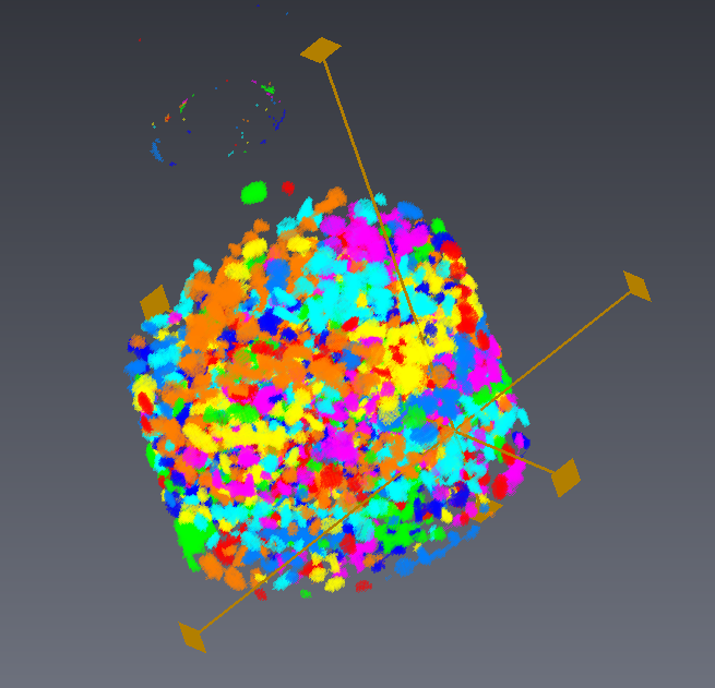
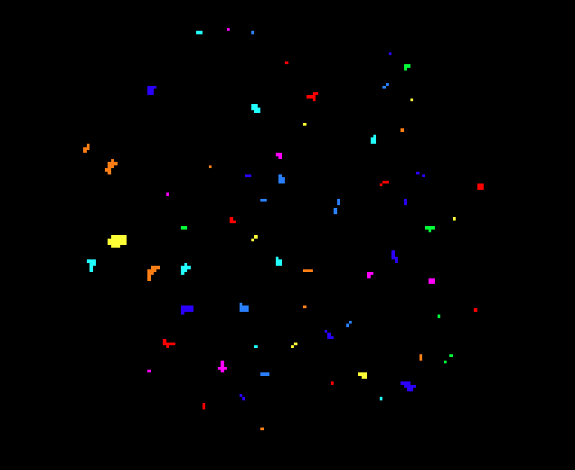
Click the Regions data object, add orthoslice to visualize. should see that each separated grain has its own color.
On the Regions data object, apply Image Morphology->Dilation to grow the outside boundary of the regions, try different kernels. You can also do dilation before connected components.
Use Display->Volume Rendering to see the grains in 3D, choose labels.am for colormap, set alpha scale to be 0.3.
Average grain size = propellant-volume / grain-number
This is how the network looks like:
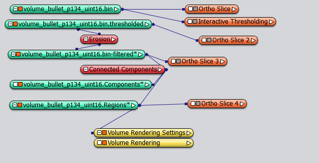
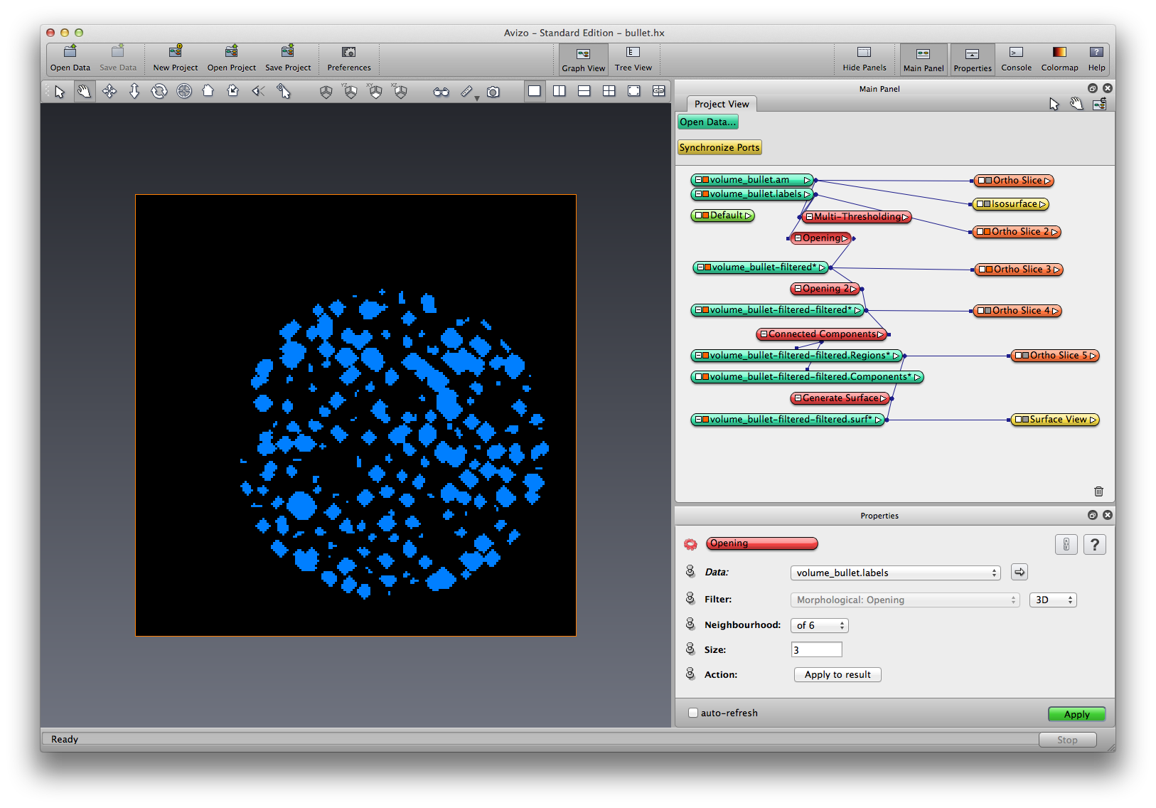
Separate the propellant grains by Morphology Opening
Right click on the .lables data object created by Multi-threshold segmentation, choose Image Morphology->Opening, set Filter to be 3D, neighborhood to be 6, size to be 3, apply. A filtered data object is created, rename it to LabelOpened-1.
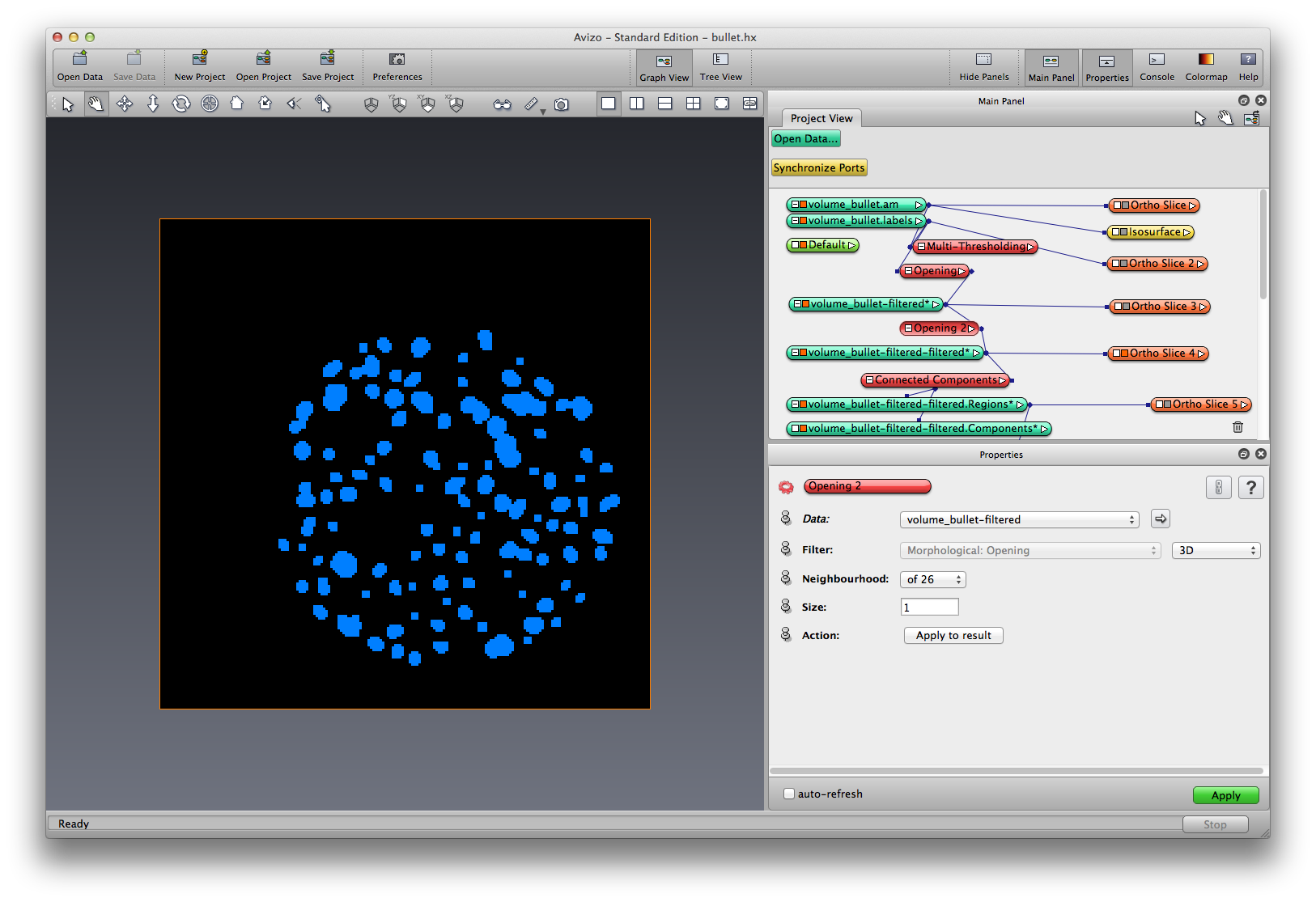
Right click on LabelOpened-1, choose Image Morphology->Opening, set Filter to be 3D, neighborhood to be 26, size to be 1, apply. Another filtered label object is created, rename it to LabelOpened-2.
Right click on LabelOpened-2, choose Image Segmentation->Connected Components, choose input as Label image, output to be both Label Image and Spreadsheet, output label image to be unsigned 16bit. apply. Two new data objects are created, a components data object, and a regions data object. Click the components data object, show the spreadsheet.
Click the Regions data object, add orthoslice to visualize. should see that each separated grain has its own color. rename the Regions data to Grains.
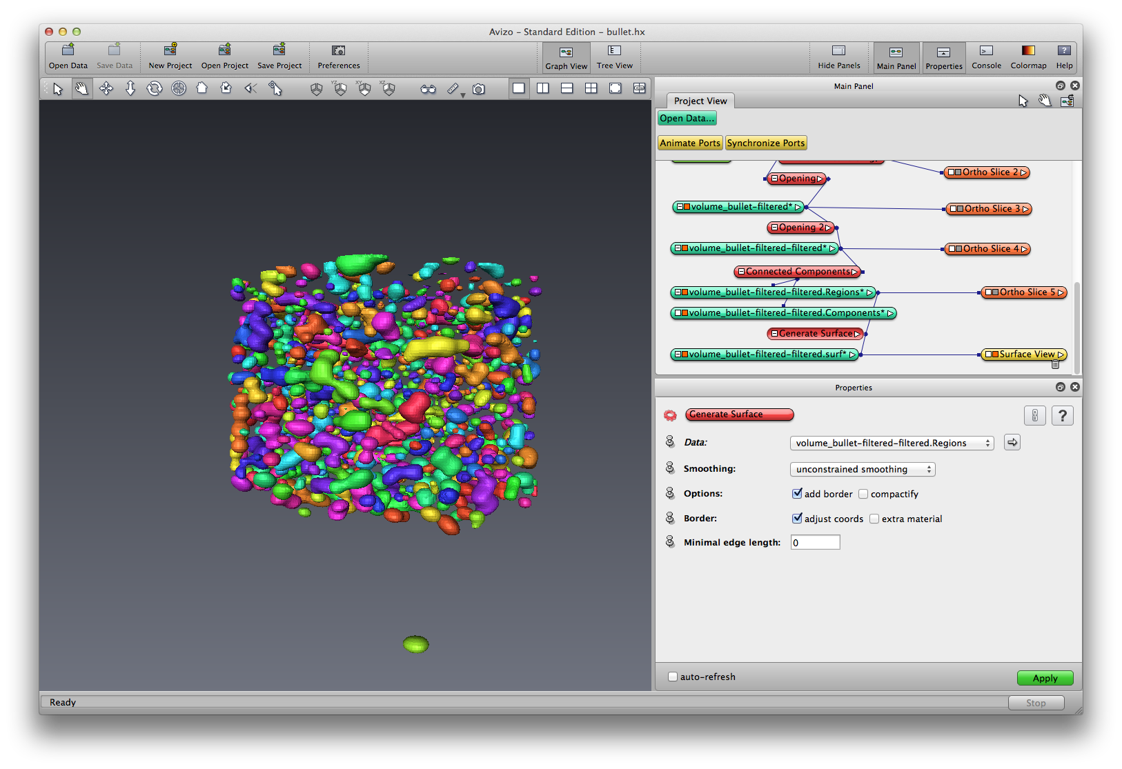
Right click on Grains, choose Compute->Generate Surface, apply, a Grains.surf data object is created, use Surface View module to visualize the grain surface in 3D.
Save your project.
Separate the propellant grains by Quantification tools
Launch Avizo 7 Fire edition, file->Open data as, choose the bullet binary dataset, click open, in the popup window, choose RAW data, click ok, input correct dataset inforamtion (243x243x227, z-fastest, little endian), click ok to load data into Avizo. A data object icon will appear in the object pool. Attach Display->orthoslice to visualize (left-click to choose the data object, then right click to choose the orthoslice module).
Attach a Quantification Tool module to data object
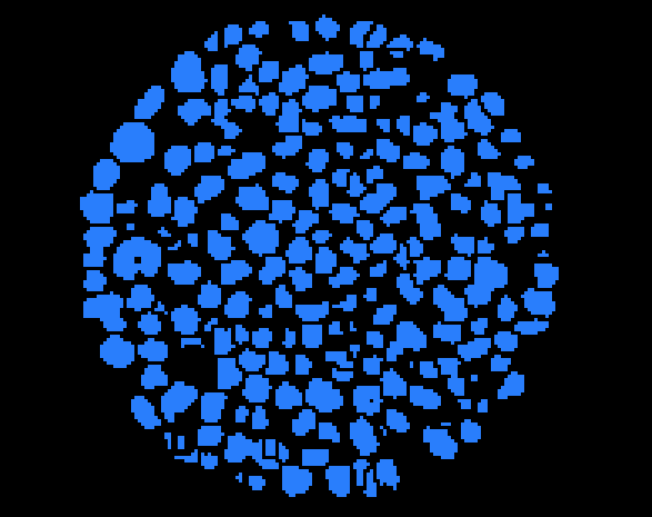
In the Quantification processing dialog, choose Thresholding->Binarisation->I_threshold, set threshold value to the range 31000-35000, Apply the threshold, a binary image is created, rename it ImageThreshold.
Attach a new or connect the existing Quantification module to ImageThreshold
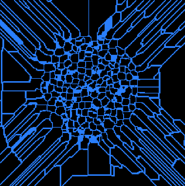
Choose Fast Morphology->Complex transforms->distxxx, leave default parameter value
Apply the distance map command, rename the result image ImageDist.
Connect the Quantification module to ImageDist, Choose Fast Morphology->Complex transforms->fastmaxima, Apply, rename the result image ImageMerged. ImageMerged is the set of most inner regions within objects.
Connect the Quantification module to ImageMerged, Choose Thresholding->Binarisation->label, Apply and rename result imageMarkers
Connect the Quantification module to ImageDist, Choose PointOperation->Logical->Logical_not, Apply and rename result image ImageDistReverse.
Connect the Quantification module to ImageDistReverse, Choose Fast Morphology->Complex transforms->fastwatershed, set second iput to imageMarkers. Apply and rename result imageWatershedLines. The watershed algorithm expand the markers toward increasing value of the reversed distance map.
Connect the Quantification module to imageThres, Choose PointOperation->Logical->Logical_sub, set the second input to imageWatershedLines. Apply and rename result imageSepGrain. This command substract the separations lines from the binary image of propellent grains.
Connect the Quantification module to imageSepGrains, Choose Thresholding->Binarisation->label, Apply and rename result image ImageGrainLabel.
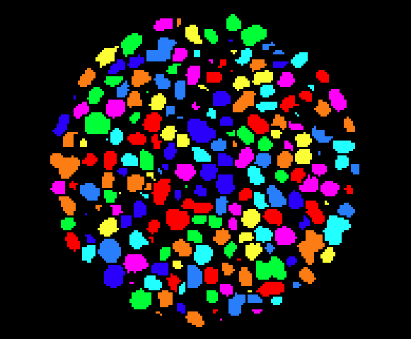
Right click on ImageGrainLabel, choose Compute->SurfaceGen, After reconstruction, you can display the resulting surface with SurfaceView module. Notice that the SurfaceGen module only works with label data.
Also notice that the resulting surface contains a large number of polygons and may require prior simplification for fast display on your hardware.
Avizo allows you to export the surfaces to various file formats, or to generate and export a tetrahedral model suitable, for instance, for finite element simulation with some external solver.
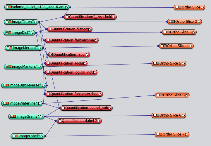
Summary: Step by step object separation by water-shed algorithm. extraction of geometric information by geometry reconstruction. The result network look like this:
Count the grains and plot grain volume distribution
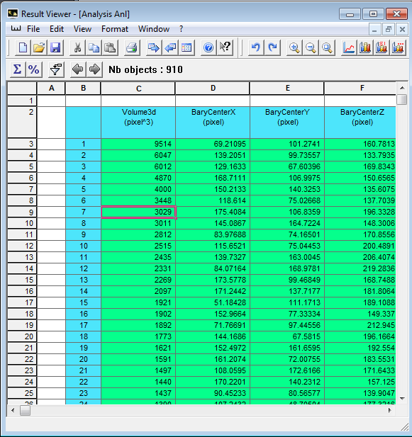
Connect the Quantification module to ImageGrainLabel, choose Analysis->Individual->I_analysis, set the second input to be the original gray-scale data, Apply, the spreadsheet result viewer appears. Each item in the spead sheet is a labeled grain volume. Click on any item in the spread sheet, a point dragger will appear in the 3D View, showing you which grain is selected. Middle mouse click on 3D view will update the dragger position, it should also find corresponding item in the spreadsheet, this didn’t work for me somehow.
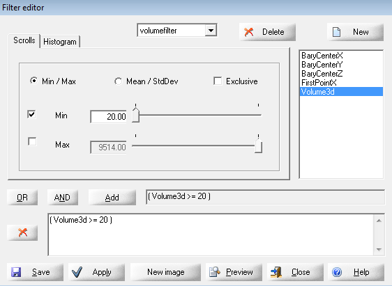
Create a filter to filter out too small grains (volume3d > 20). Apply, the results will be updated.
click the sum tool in the result viewer to get the min, max, mean, stddev, and sum of all the grains. Try to compute average grain size from the numbers you get here.
Choose some measurements, such as volume, try to plot them into different graph styles. on the menu bar, choose Window->Analysis Anl1 to go back to spreadsheet style. Click the excel icon to export measuments to a Microsoft Excel sheet. If you want to customize your measurement, on menu bar, choose View->Measure bar, so the measure toolbar appears, and click on measure selection icon. We’ll not do it here, you can practice by yourself.