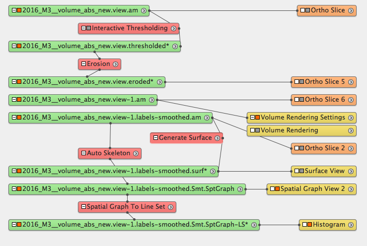
Auto skeleton

Dataset: 2016_M3_bin2

Crop data

The original data is 800x800x700. At Z-direction, it’s cropped to keep index 92-654, to eliminate bad slices

Remove noise surrounding the sample

Remove noise is achieved by creating mask:

1. original slice

   

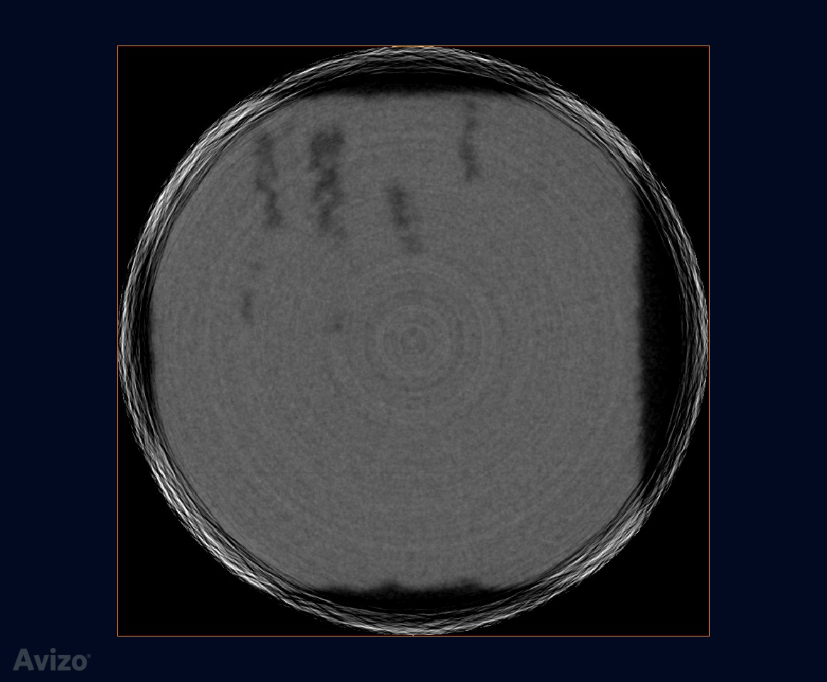
2. interactive thresholding

   

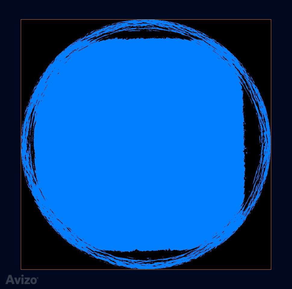
3. erosion: tried 3D size 5, or XY planes size 9, both works –> create a clean mask

   

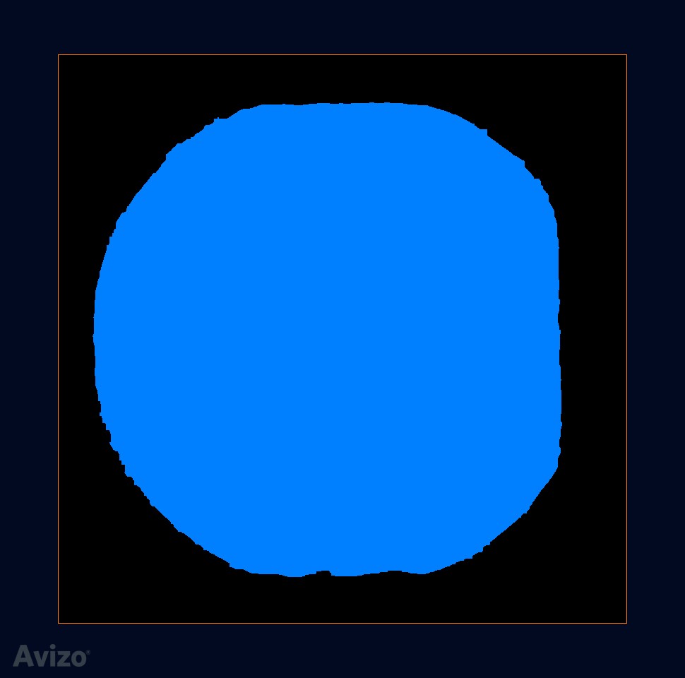
4. arithmetic: data * mask –> create clean data

Volume rendering

Adjust the data window to show cracks. The important thing is to edit the colormap, so the color beyond data range is transparent.

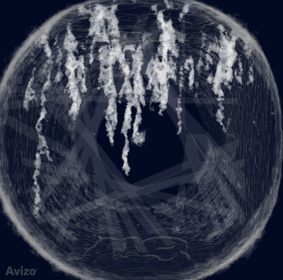
Notice the bad slices widened after aggressive erosion

Segment the cracks

I used segmenation editor, magic wand + all slices. Then remove noise from menu segmentation -> smooth labels ...

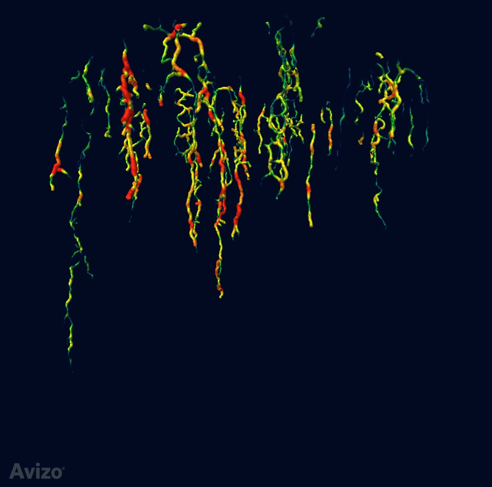
Auto Skeleton

Attach to crack segmentation. Use default parameters. In “Spatial graph view”, show segments, tubes, scale by thickness, color by thickness (thickness min-max: 0.5-12.1 colormap: blue to red)

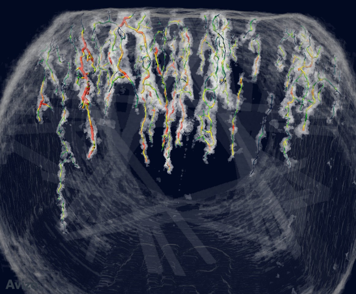
Show against volume rendering:

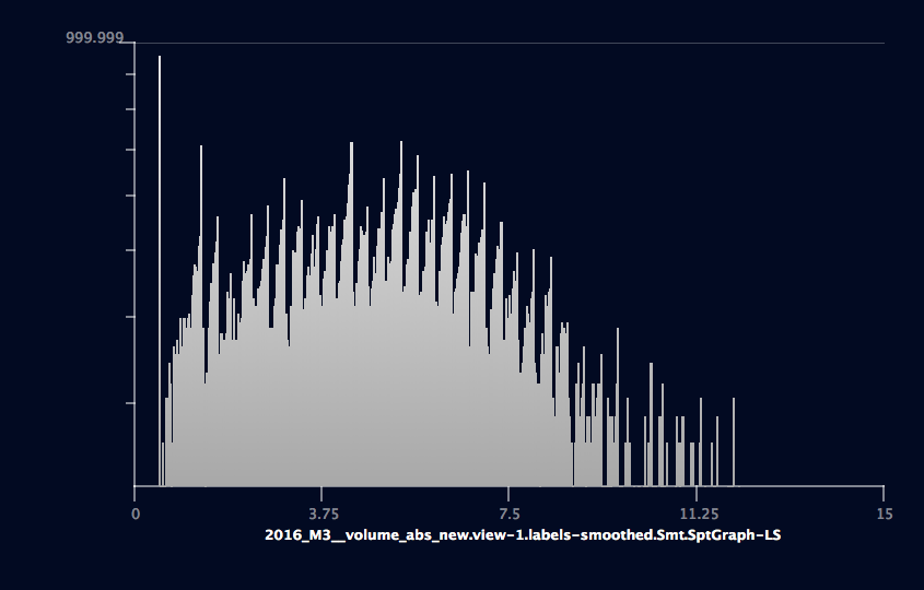
Thickness histogram

The SpatialGraph data can be converted to lineset. Then plot histogram on the lineset data. Choose “data 0” on “data channel” port. Click “Reset” button on “Range” port to reset data min-max. The lineset includes total 12678 points, with xyz coordinates and thickness data. The total line (segment) number is 539

Avizo network